2.3 Error definition criteria
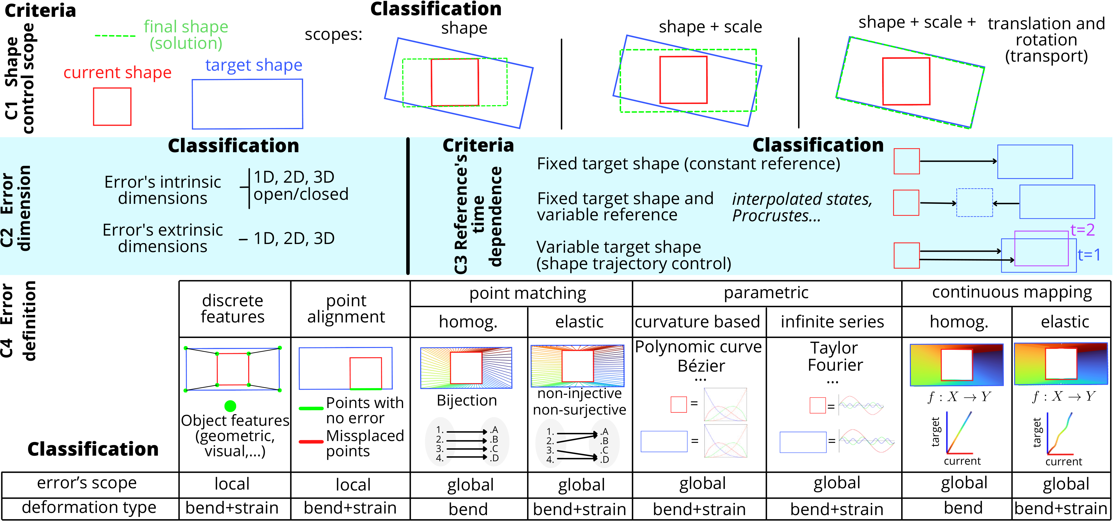
Table 3. Criteria from Sec. IIC applied to several shape control methods. Abbreviations: pos. (position), targ. (target), ref. (reference) and desc. (descriptor).
| Method | C1 Shape control scope | C2 Error dimensionality | C3 Reference's time dependence | C4 Error definition | |
|---|---|---|---|---|---|
| (Aranda et al., 2020) | Shape + scale + transport | 2D intrinsic, 3D extrinsic | Fixed targ., variable ref. | Discrete features, RMS error | |
| (Shetab-Bushehri et al., 2022) | Shape + scale + transport | Discrete points pos. | Constant | Mesh point matching | |
| (Qi et al., 2022) | Shape + scale + transport | Discrete points pos. | Constant | Homogeneous contour mapping | |
| (Cui et al., 2020) | Shape + scale | Discrete points pos. | Constant | Discrete feature points alignment | |
| (J. Zhu et al., 2021) | Shape + scale | Discrete points pos. | Fixed targ., variable ref. | Homogeneous contour mapping | |
| (A. Cherubini et al., 2020) | Shape | Image pixels | Constant | Point (pixel) alignment | |
| (López-Nicolás et al., 2020) | Shape + scale + transport | Discrete points pos., 2D | Constant | Homogeneous contour mapping | |
| (Hu et al., 2019) | Shape + scale | Discrete points pos., 30 feature desc. | Constant | Discrete features (FPFH) alignment | |
| (Cuiral-Zueco and López-Nicolás, 2021) | Shape + scale | 1D intrinsic, 3D extrinsic | Fixed targ., variable ref. | Elastic contour point matching | |
| (Cuiral-Zueco et al., 2023) | Shape | 1D intrinsic, 2D extrinsic | Constant | Elastic contour mapping | |
| (Cuiral-Zueco and López-Nicolás, 2024) | Shape + scale | 2D intrinsic, 3D extrinsic | Fixed targ., variable ref. | Homogeneous surface mapping | |
| (Caporali et al., 2024) | Shape + scale + transport | 1D intrinsic, 3D extrinsic | Fixed targ. | Homogeneous curve map | |
| (Deng et al., 2024) | Shape + scale + transport | 2D intrinsic, 3D extrinsic | Fixed targ., variable ref. | Homogeneous shape point matching |
The concept of shape lacks standard mathematical formalisation (see (Arriola-Rios et al., 2020) for several shape-representation methods). This leads authors to use a variety of approaches in order to infer shape error between the manipulated and desired shapes of the object. This diversity underlines the need to include a classification of shape comparison and error definition in this taxonomy (see Fig. 4 and Table 3).
Consider a shape representation (e.g., geometric descriptors, the contour's curvature, etc.) of the manipulated object \(\mathcal{S}(t, u(t))\), where \(u(t)\) denotes manipulation actions, and the corresponding shape representation of the desired target shape \(\mathcal{S}_\mathrm{t}(t)\). Omitting time dependence, let \(\Pi(\mathcal{S}_\mathrm{t}) = \mathcal{S}\) denote the correspondence of elements of \(\mathcal{S}_\mathrm{t}\) to elements of \(\mathcal{S}\) (e.g., feature correspondences, a contour map, etc.). Additionally, consider a shape error metric \(E(\mathcal{S}, \Pi(\mathcal{S}_\mathrm{t}))\) (for a formal definition of shape metric see (Al-Aifari et al., 2013)) that measures the similarity between shapes \(\mathcal{S}\) and \(\mathcal{S}_\mathrm{t}\) under the correspondences established by \(\Pi\) (e.g., Euclidean distance between matched discrete features, curvature differences between mapped contours, etc.). We formulate the fundamental shape control problem as: \[ \min_{u} E(\mathcal{S}(u), \Pi(\mathcal{S}_\mathrm{t})) \; (1), \] The formulation above is the fundamental starting point from which additional considerations and constraints can be defined (those are classified in Section 2.4). Considering (1) we now categorise shape error definition with 4 criteria.
2.3.1 Shape control scope
2.3.2 Error dimensionality
2.3.3 Reference's time dependence
2.3.4 Error definition types
The last criterion we introduce for the error characterisation is the error definition through shape comparison, that is, how the correspondence \(\Pi(\mathcal{S}_\mathrm{t})=\mathcal{S}\) between shape representations is defined in order to compute \(E(\mathcal{S}, \Pi(\mathcal{S}_\mathrm{t}))\) in (1). For this, we propose a set of 8 categories (criterion C4 in Fig. 4). Note that our focus is not on the definition of specific shape representations \(\mathcal{S}\) or \(\mathcal{S}_\mathrm{t}\), something covered in depth in (Arriola-Rios et al., 2020)), but rather on the methods that facilitate a proper comparison of such shape representations (i.e., \(\Pi\) in (1)).
Our error classification ranges from discrete to continuous methods, starting with discrete feature-based errors that compare sparse visual or geometric features of an object to its target shape, without fully representing the object's geometry. Errors based on point alignment focus on points that align with the target, and are effective for local but not global deformations. For global geometric errors, shape point matching techniques, classified into homogeneous (uniform distribution of points) and elastic (variable spatial density) matching, provide a holistic approach to shape errors for bending and strain deformations, respectively. In addition, parametric errors based on curves (e.g., Bézier curves) or infinite series (e.g., Fourier series or Laplace-Beltrami eigenfunctions) focus on the comparison of the mathematical parameters that define the shapes. We also present errors based on continuous maps, similar to their discrete counterpart (shape point matching). They are divided into homogeneous (e.g., functional maps) and elastic (e.g., Fast Marching Method based mapping). Elastic continuous maps are particularly suitable for strain deformation processes.