This work was supported via project REMAIN - S1/1.1/E0111 (Interreg Sudoe Programme, ERDF), and via projects PID2021-124137OB-I00 and TED2021-130224B-I00 funded by MCIN/AEI/10.13039/501100011033, by ERDF A way of making Europe and by the European Union NextGenerationEU/PRTR.
5 Simulation Results
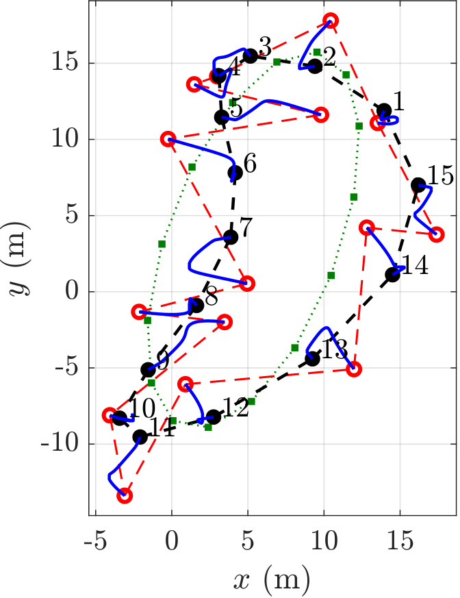
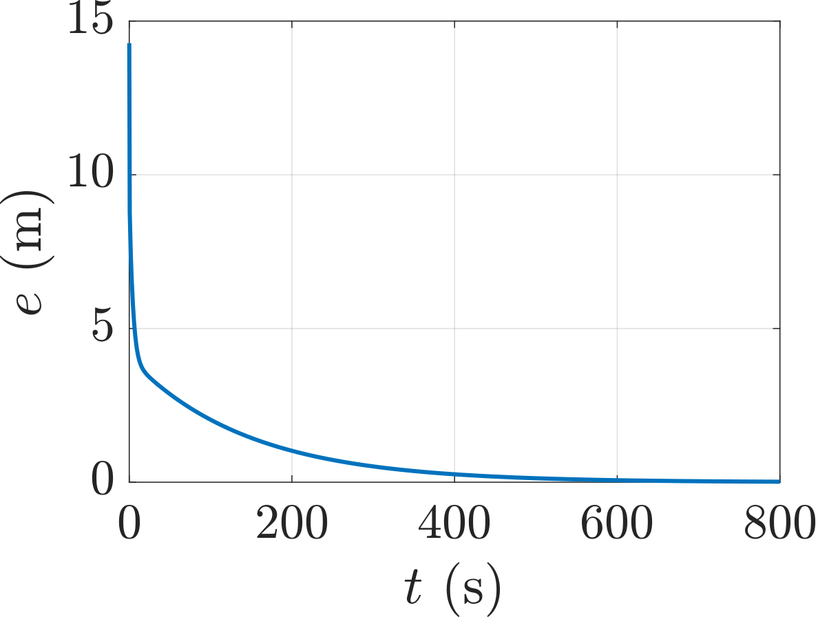
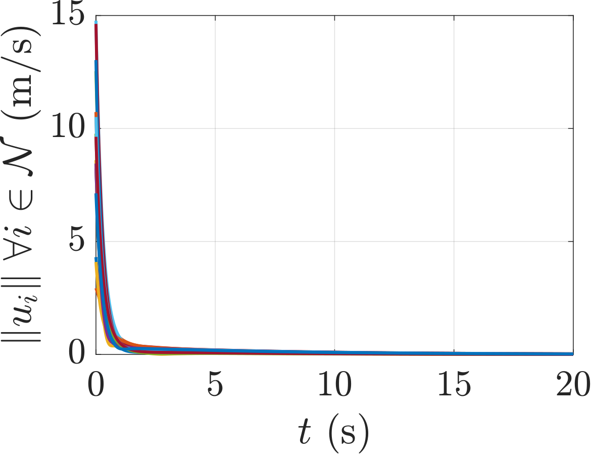
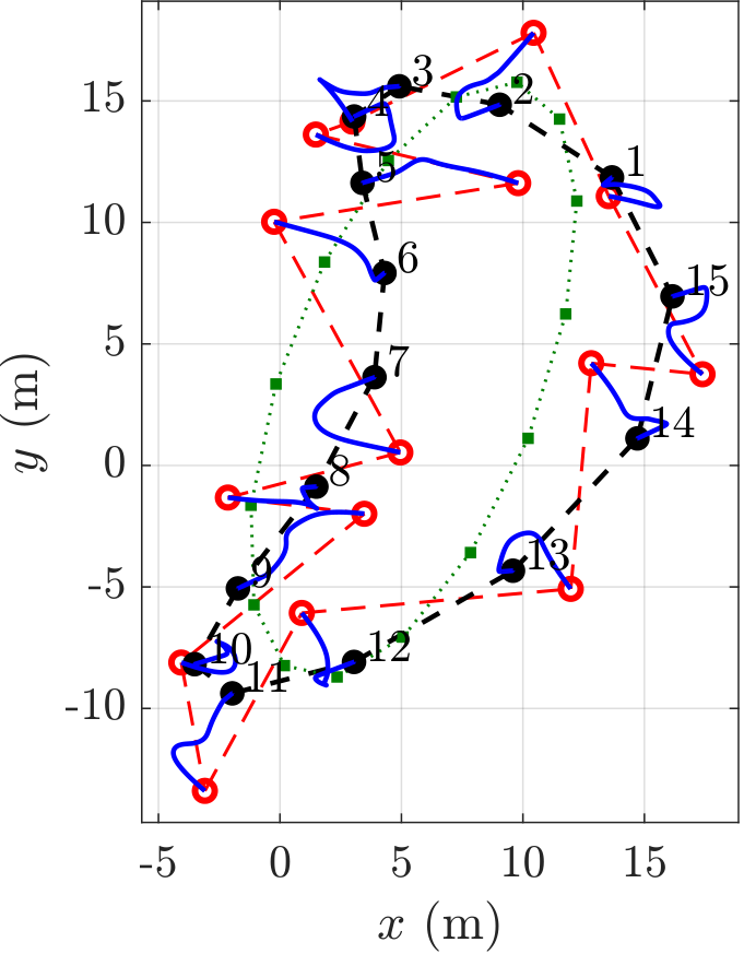
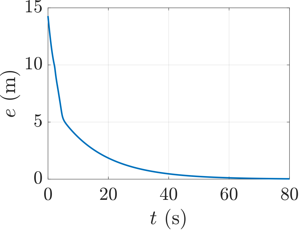
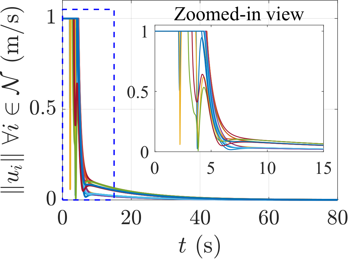
Figure 2. The three plots at the top show the results with the original control law. The three at the bottom show the results with saturation and higher gain. Left plots: initial agent positions (red hollow circles), final agent positions (black solid circles), agent paths (blue solid lines). Agent indices and dashed lines joining consecutive agents are also shown. The final positions if using only one nominal configuration are shown as small green squares. Right plots: error metric (top) and velocity norms (bottom) over time.
We illustrate our approach via numerical simulation in MATLAB. The task is for the agents to form a low-frequency discretized 2D closed curve (M. Aranda, 2023; M. Aranda et al., 2024). By avoiding high frequencies, such a curve avoids sharp local variations and preserves physical agent vicinities, while having a highly flexible shape. These are useful features for, e.g., enclosing a phenomenon taking place in the interior of the curve. We use a discrete Fourier-based representation of planar closed curves with two low-frequency components. The nominal configurations are Fourier basis vectors at these frequencies. We build \(C\) in (4) as follows, where the arguments have the form \(k \frac{2\pi (i-1)}{N}\) with \(k\) indexing the frequency and \(i\) the agent:
\[
C= \begin{bmatrix}
\cos(1 \frac{2\pi\cdot 0}{N}) & \cos(1 \frac{2\pi\cdot 1}{N}) & \cdots & \cos(1 \frac{2\pi\cdot (N-1)}{N}) \\
\sin(1 \frac{2\pi\cdot 0}{N}) & \sin(1 \frac{2\pi\cdot 1}{N}) & \cdots & \sin(1 \frac{2\pi\cdot (N-1)}{N})\\
\cos(2 \frac{2\pi\cdot 0}{N}) & \cos(2 \frac{2\pi\cdot 1}{N}) & \cdots & \cos(2 \frac{2\pi\cdot (N-1)}{N}) \\
\sin(2 \frac{2\pi\cdot 0}{N}) & \sin(2 \frac{2\pi\cdot 1}{N}) & \cdots & \sin(2 \frac{2\pi\cdot (N-1)}{N})\\ 1 & 1 & \cdots & 1
\end{bmatrix}^\intercal.
\]
Note that we have \(L=2\) and \(M=D\cdot L+2=6\). We take \(N=15\) and use a closed chain structure with \(N_s=N\) sets \(\mathcal{S}_j\). For every \(G_j\), the determinant is \(8.26 \cdot 10^{-3}\) and the condition number is \(3.15 \cdot 10^{2}\). Therefore, Assumption 1 is satisfied. To assess formation achievement, we use the error metric \(e(t) = \| (I_{D\cdot N} - (C \otimes I_D) (C \otimes I_D)^+)p(t) \|\) which expresses the distance from \(p(t)\) to the column space of \(C \otimes I_D\). We simulate our control law, using the time step \(0.01\) s. Fig. 2 illustrates the convergence of the multiagent team toward a low-frequency discretized closed curve. We run again the same test incorporating a multiplicative control gain equal to \(10\) for every agent and saturation of every \(\|u_i(t)\|\) at \(1\) m/s. As seen in the plots, this improves the convergence behavior, which is influenced by matrix conditioning. The configuration \(p(t\rightarrow \infty)\) depends on the initial state \(p(0)\) and the system dynamics, and is not controlled in our approach.
Taking only the frequency index \(k=1\), i.e., a single nominal configuration with the geometry of a discretized circle, the achievable final configurations would be limited to discretized ellipses, as seen in the figure. This is because an ellipse is an affine transformation of a circle. By using two nominal configurations, our approach allows the team to acquire more complex shapes than an ellipse while still forming a low-frequency closed curve. This increases flexibility during enclosing. Using different nominal configurations (not Fourier-based) would offer different properties, while retaining our core advantage: allowing a wider range of achievable shapes than affine formation control in its standard form (i.e., with a single and constant nominal configuration).