Manuscript received March 10, 2023; Accepted June 23, 2023. This paper was recommended for publication by Editor P. Vasseur upon evaluation of the Associate Editor and Reviewers' comments.
This work was supported via projects PID2021-124137OB-I00 and TED2021-130224B-I00 funded by MCIN/AEI/10.13039/501100011033, by ERDF A way of making Europe and by the European Union NextGenerationEU/PRTR. This work was also partially supported by the Wallenberg AI, Autonomous Systems and Software Program (WASP) funded by the Knut and Alice Wallenberg Foundation.
4 Experiments
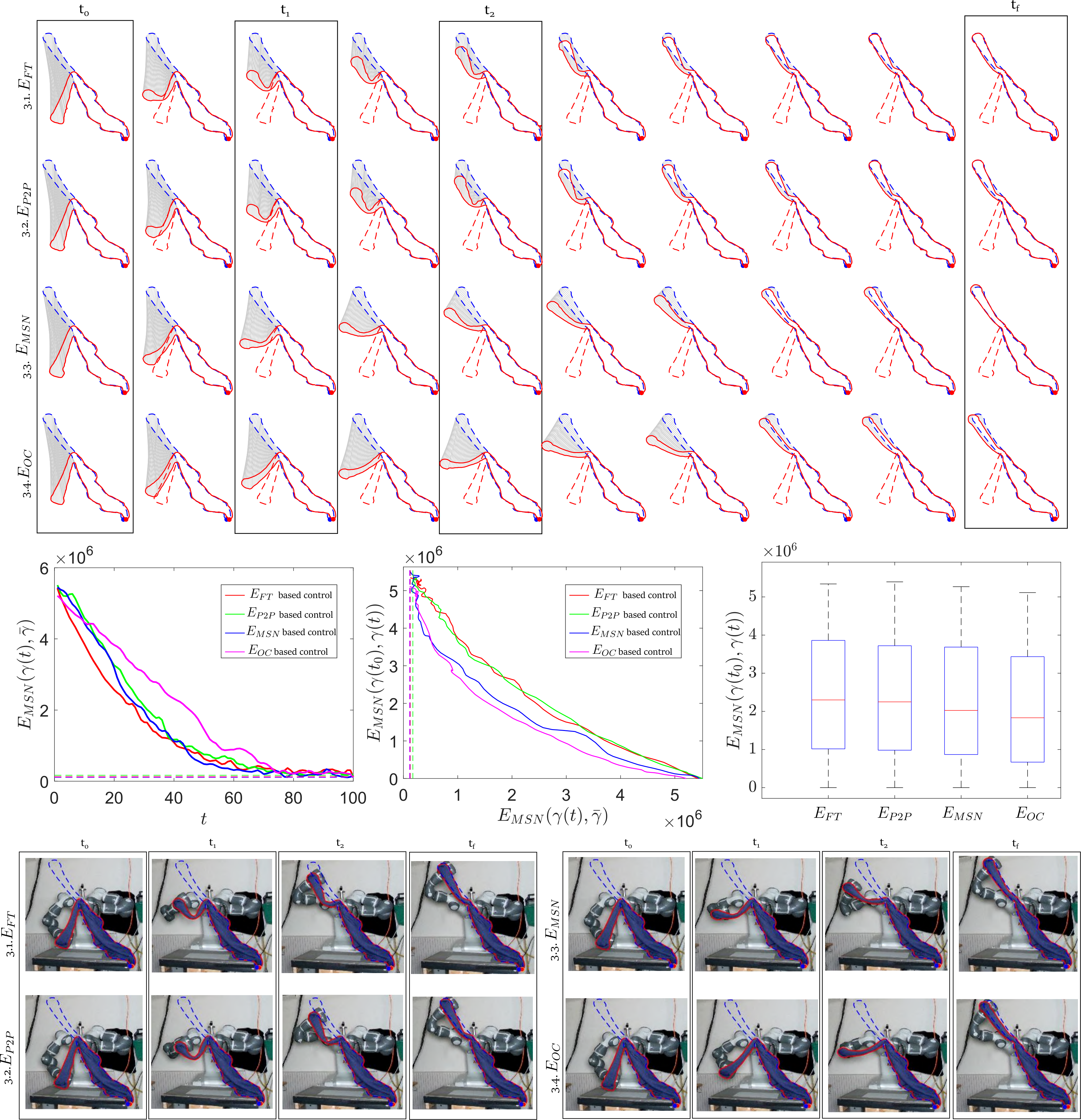
Figure 6. Four experiments involve shape control of a sweater (right gripper is fixed). The object-compliant performance of four shape control strategies is compared, reducing respectively \(E_{\mathrm{FT}}\) (Exp. 3.1), \(E_{\mathrm{P2P}}\) (Exp. 3.2), \(E_{\mathrm{MSN}}\) (Exp. 3.3) and \(E_{\mathrm{OC}}\) (Exp. 3.4). Experiment 3.4 reduces \(E_{\mathrm{OC}}\) (10) with \(\beta=1\) and \(r_{\mathrm{OC}}=0.1r_{\rm{max}}\) thus penalising relatively local deformations. Elements in graphs and plots are introduced in the description of Fig. 3 except for the box-plot on the right, which represents the deformation cost distribution of each strategy according to \(E_{\mathrm{MSN}}(\gamma(t_0),\gamma(t))\). First plot (left) shows how all strategies lead to similar final absolute error values. In the middle plot, Exp. 3.4 leads to the lowest deformation path (purple line). This is shown in the shape evolution sequences (above), where Exp. 3.4 generates almost no changes in the local curvature of the shape besides the bending in the pivoting region (centre of the object). The equivalence of \(E_{\mathrm{P2P}}\) and \(E_{\mathrm{FT}}\) (lemma ref) is exemplified in Exp. 3.1 and Exp. 3.2: both extrinsic energies follow similar shape evolution paths (middle plot), generate large deformations and, unlike Exp. 3.3 and Exp. 3.4, lead to curvature error in the middle part of the object (see the \(t_{f}\) instants above).
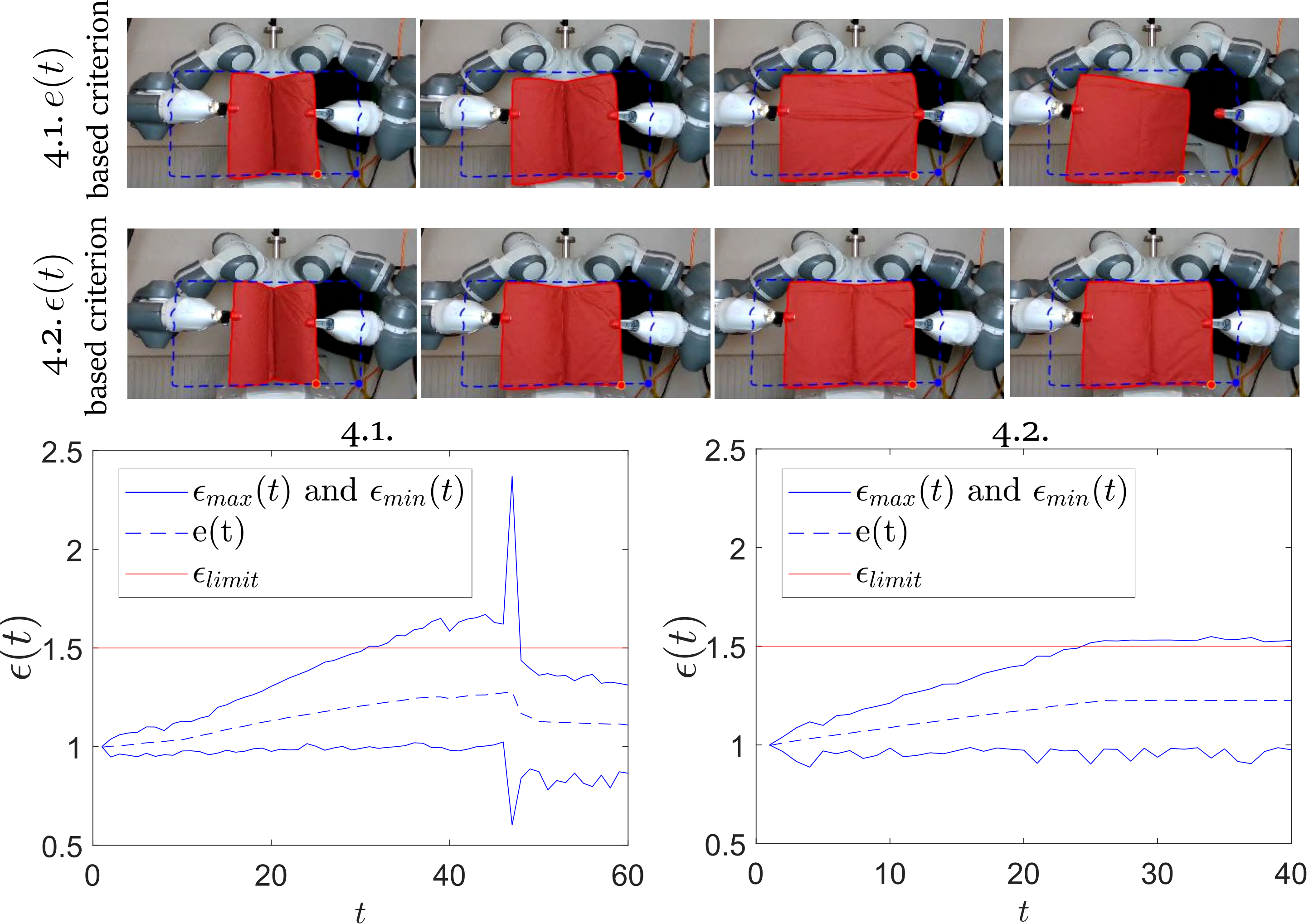
The first group of experiments (Fig. 6) compares the performance of a Jacobian-based control law applied to four different energies, particularly \(E_{\mathrm{P2P}}, E_{\mathrm{FT}}, E_{\mathrm{MSN}}\) and \(E_{\mathrm{OC}}\) (Exp. 3.1 to 3.4, respectively). The extrinsic shape energies \(E_{\mathrm{FT}}\) and \(E_{\mathrm{P2P}}\) lead to larger deformation paths (i.e., equivalent paths, lemma ref), whereas the strategy that seeks reducing \(E_{\mathrm{OC}}\) leads to lower deformation. Note time instant \(t_1\) where, if instead of cloth a thin metal sheet was being deformed, \(E_{\mathrm{MSN}}\) would likely lead to high compression and higher chances of bucking, whereas \(E_{\mathrm{OC}}\) generates a less aggressive shape evolution. In experiment 3.4, the solution trajectory of the robot arm performs a longer circular arch, thus leading to a slightly slower performance. Further analysis is presented in the description of Fig. 6. Experiments 4.1 and 4.2 in Fig. 7 illustrate the performance of (12) as an approximation of a local strain measure. They compare \(e(t)\) (Exp. 4.1) and \(\epsilon(t)\) (Exp. 4.2) as approximations of an object's strain (with strain limit 1.5 as input information). Measure \(e(t)\) leads to an over-stretching action that causes gripper failure. On the other hand, \(\epsilon(t)\) allows to properly stop the process thus preventing failure (see description on Fig. 7 for more insights).
Figure 7. Stretching process of a cardboard piece towards an unfeasible target shape that requires over-stretching the object. In the plots, average values \(\epsilon_{avg}(t)\equiv e(t)\), maximum \(\epsilon_{{max}}(t)\) and minimum \(\epsilon_{min}(t)\) values of \(\epsilon(s,t)\) with respect to \(s\) are plotted, hence the dependence on \(s\) has been removed from the y-axis label. The system receives as input the strain limit of \(\epsilon_{limit}=1.5\). In Exp. 4.1 the strain is measured through e(t) whereas in Exp. 4.2 \(\epsilon(t)\) is used as local strain measure. This task involves unevenly distributed contour length changes: vertical sides of the shape do not change their length. In Exp. 4.1, Strain measure \(e(t)\) does not perceive the limit \(\epsilon_{limit}=1.5\) being reached, thus the object is over-stretched leading to grip failure: note the abrupt change in plot 4.1 (around second 45). Local strain measure \(\epsilon_{{max}}(t)\) in Exp. 4.2 allows to stop the control when the strain limit is reached. Note that \(\epsilon(t)\) also allows (through \(\epsilon_{min}(t)\)) to consider the maximum local compression that takes place on the object.