2 Geometry-based deformation energy
2.1 Proposed multi-scale normal (MSN) energy: $E_{\mathrm{MSN}}$
In this section we present a geometry-based deformation energy for OCSC. In texture-less objects, the only visual indicators of objects undergoing deformations are the local changes in length and curvature of their contour. We therefore define our analysis using these two key elements.
Our proposed energy relies on a shape representation analogous to the discrete multi-scale Laplacian descriptors presented in (Cuiral-Zueco and López-Nicolás, 2021) for elastic contour mapping. We define a continuous multi-scale normal (MSN) shape representation that provides a notion of multi-scale mean curvature. We make use of geodesic balls \(B(s,r)\subseteq \gamma(s)\) centred at \(s\) with radius \(r\in(0,r_{\rm{max}}]\subset\mathbb{R},\) (Fig. 2), being \(r_{\rm{max}}=l(t)/2\) and \(l(t)\in\mathbb{R}\) the total contour length. In this paper we will refer to radius \(r\) as scale of analysis (or simply scale). A scale defines the neighbouring region (i.e., the scope of analysis) at a given point \(s\). Therefore, our proposed shape representation \(\mathbf{l}(s,r)\in\mathbb{R}^2\) is obtained as \[ \mathbf{l}(s,r)=-\frac{1}{{r}}\int_{B(s,r)}\mathbf{x}^{\Re(s)}(s')\mathrm{d}l, \tag{1} \] where \(\mathbf{x}^{\Re(s)}(s')=(x^{\Re(s)}(s'),y^{\Re(s)}(s'))^\intercal\in\mathbb{R}^2\) are the extrinsic position vectors of points corresponding to parameter values \(s'\in B(s,r)\) and expressed in the reference \(\Re(s)\). Element \(\mathrm{d}l\) in (1) is the differential element of contour length \(l(t)\). As \(r\rightarrow 0\), (1) leads to the curvature weighted normal vectors (referred to \(\Re(s)\)). Coordinates of points within the integration domain are still expressed from frame \(\Re(s)\not\equiv \Re(s')\) and, therefore, descriptors \(\mathbf{l}(s,r)\) constitute both intrinsic and extrinsic descriptors (Bronstein et al., 2007).
Consider \(\bar{s}=\Pi(s,t)\) where \(\Pi(s,t):\gamma(t)\rightarrow \bar{\gamma}\) is an elastic map (diffeomorphism) that maximises multi-scale curvature similarity between contours. Using the shape representation (1), we define shape error \(\mathbf{e}_{\mathrm{MSN}}\) as \[ \mathbf{e}_{\mathrm{MSN}}(s,r,t)=\mathbf{l}(s,r,t)-\bar{\mathbf{l}}(\Pi(s,t),r), \tag{2} \] where \(\bar{\mathbf{l}}(\Pi(s,t),r)\) constitutes the multi-scale normal (MSN) descriptor of the target shape at point \(\Pi(s,t)=\bar{s}\). Using error (2) we introduce our proposed geometry-based deformation energy as: \[ E_{\mathrm{MSN}}(\gamma(t),\bar{\gamma})=\begin{matrix} \\ \text{min} \\ \Pi \end{matrix} \int_{0}^{l(t)}\int_{0}^{r_{\rm{max}}}\mathbf{e}_{\mathrm{MSN}}^\intercal\mathbf{e}^{}_{\mathrm{MSN}}\mathrm{d}r\mathrm{d}s, \tag{3} \] where \(l(t)\) is the length of curve \(\gamma(t)\). The optimisation process for obtaining \(\Pi\) in 1D domains can be performed by means of the Fast Marching Method (as proposed in (Cuiral-Zueco and López-Nicolás, 2021)).
2.2 Characteristics of $E_{\mathrm{MSN}}$ as a shape metric
Energy \(E_{\mathrm{MSN}}\) quantifies differences between shapes through their geometric features as it constitutes a metric in shape space as defined in (Al-Aifari et al., 2013). That is, considering three shapes \(\gamma_1, \gamma_2\) and \(\gamma_3\):
\[ \begin{split} E_{\mathrm{MSN}}(\gamma_1,\gamma_2)=E_{\mathrm{MSN}}(\gamma_2,\gamma_1), \\ E_{\mathrm{MSN}}(\gamma_1,\gamma_2)=0\,\Rightarrow \gamma_1\equiv \gamma_2, \\ E_{\mathrm{MSN}}(\gamma_1,\gamma_3)\leq E_{\mathrm{MSN}}(\gamma_1,\gamma_2)+E_{\mathrm{MSN}}(\gamma_2,\gamma_3). \end{split} \]
Some relevant features of metric \(E_{\mathrm{MSN}}\) for OCSC are:
2.2.1 Invariance to SE(2)
2.2.2 Multi-scale scope
2.2.3 Use of elastic mapping
2.2.4 Joint intrinsic-extrinsic metric
\(E_{\mathrm{MSN}}\) is intrinsic, since it is defined by geodesic distances and local coordinates, and extrinsic, as it is based on the multi-scale mean normal curvature obtained from the extrinsic analysis of domains \(B(s,r)\). In shape control, a conventional approach is to minimise extrinsic energies that disregard the object's topology. The joint intrinsic-extrinsic nature of \(E_{\mathrm{MSN}}\) makes it aware of topology changes and non-isometric deformations (Bronstein et al., 2007) leading to gentler deformation paths.
2.3 Extrinsically-defined shape energies
In this section, we revisit general definitions of the conventional extrinsic shape energies \(E_{\mathrm{P2P}}\), used in (López-Nicolás et al., 2020), (Berenson, 2013), (Cuiral-Zueco and López-Nicolás, 2021), (Shetab-Bushehri et al., 2022) or (Aranda et al., 2020), and \(E_{\mathrm{FT}}\), used in (Navarro-Alarcon and Liu, 2017). We endow them with elastic maps in order to fairly compare their performance with our proposed energy \(E_{\mathrm{MSN}}\) in upcoming sections.
The point-to-point (P2P) error, endowed with an elastic map \(\Pi\), can be formulated as: \[ \mathbf{e}_{\mathrm{P2P}}(s,t)=\mathbf{x}(s,t)-\left(\mathbf{R}^*\bar{\mathbf{x}}(\Pi(s,t))+\mathbf{t}^*\right), \tag{4} \] where \(\mathbf{x}(s,t),\bar{\mathbf{x}}(\Pi(s,t))\in\mathbb{R}^2\) are the extrinsic coordinates of the current and target contour points respectively. Transform \((\mathbf{R}^*, \mathbf{t}^*)\) is the orthogonal Procrustes rigid transform (Al-Aifari et al., 2013) that, by removing the rigid translation and rotation component from the point-to-point error, minimises the energy: \[ E_{\mathrm{P2P}}(\gamma(t),\bar{\gamma})=\begin{matrix} \\ \text{min}\\ \mathbf{R}^*,\mathbf{t}^*,\Pi \end{matrix} \int_{0}^{l(t)}\mathbf{e}_{\mathrm{P2P}}^\intercal\mathbf{e}^{}_{\mathrm{P2P}}\mathrm{d}s. \tag{5} \] Alternatively, energy \(E_{\mathrm{FT}}\) is defined in the frequency domain through the Fourier Transform. Consider the complex function \(z(s)=x(s)+y(s)i\), where the \(x(s)\) coordinates of \(\gamma(s)\) constitute the real term and the \(y(s)\) coordinates the imaginary term. The complex Fourier coefficients \(c_n,\bar{c}_n\) obtained from \(z(s),\bar{z}(\Pi(s))\) lead to the Fourier-based energy: \[ E_{\mathrm{FT}}(\gamma(t),\bar{\gamma})=\begin{matrix} \\ \text{min} \\ \Pi \end{matrix}\sum_{n=-\infty}^{\infty}\left | c_n-\bar{c}_n \right |^2. \tag{6} \] Note that the summation bounds in (6) can be truncated thus allowing to filter out high frequency (nosiy) components.
Shape energies \(E_{\mathrm{P2P}}\) and \(E_{\mathrm{FT}}\), defined in (5) and (6) respectively, are equivalent (up to a Procrustes transform).
The proof follows from the direct application of Parseval's Theorem (Parseval, 1806) to (6): \[ \sum_{n=-\infty}^{\infty}\left | c_n-\bar{c}_n \right |^2 =\int_{0}^{l(t)}\left | z(s)-\bar{z}(\Pi(s)) \right |^2 \mathrm{d}s \\ =\int_{0}^{l(t)}\| \mathbf{x}(s)-\mathbf{\bar{x}}(\Pi(s)) \|^2 \mathrm{d}s= \int_{0}^{l(t)}\mathbf{e}_{\mathrm{P2P}}^\intercal\mathbf{e}^{}_{\mathrm{P2P}}\mathrm{d}s. \tag{7} \]
2.4 Validation of $E_{\mathrm{MSN}}$ for OCSC
In this section we validate \(E_{\mathrm{MSN}}\), through experiments and simulations, as a metric that allows to quantify deformation and as a shape error that produces lower deformation paths in shape control.
The experiments presented along this paper are performed on the ABB Yumi dual-arm robot using colour-based object segmentation (in CIELAB colour space) and \(\alpha\)-shape contour extraction. The continuous elastic contour map \(\Pi(s,t)\) is computed as in (Cuiral-Zueco and López-Nicolás, 2021) and then sampled to interpolate values of \(\bar{\mathbf{l}}(\bar{s},r)\) in (2) with sub-pixel resolution. We avoid using any specific Jacobian update-rules (as in (Zhu et al., 2021) or (Navarro-Alarcon and Liu, 2017)) in order to compare the different energies as consistently as possible: Jacobians are experimentally estimated throughout the whole process in all the experiments.
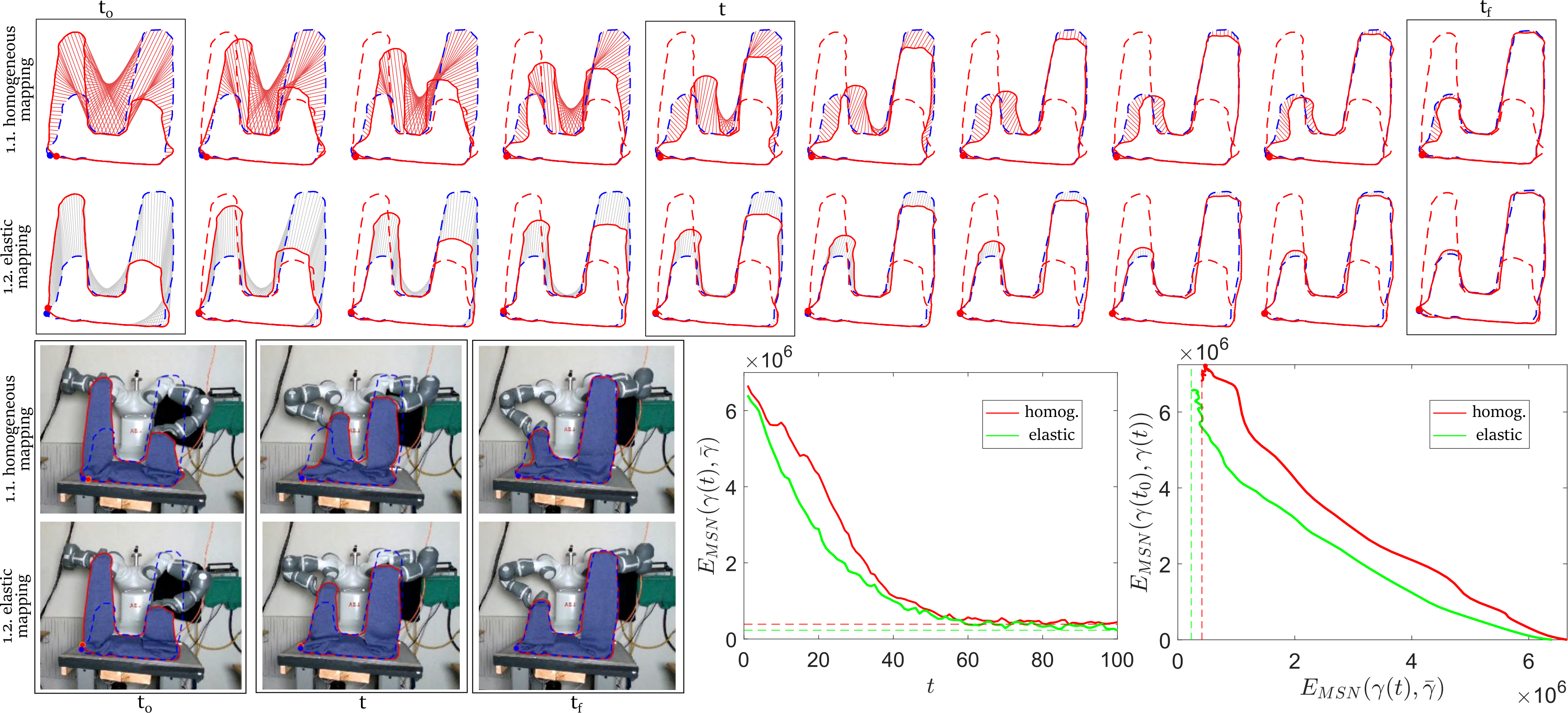
To illustrate the performance of \(E_{\mathrm{MSN}}\) as a deformation measure, we use it to analyse the results of experiments 1.1 and 1.2 (Fig. 3). Both experiments involve the reduction of the shapes' Fourier-based spectral energy. However, Exp. 1.1 uses a homogeneous contour mapping, whereas Exp. 1.2 uses elastic mapping (i.e., \(E_{\mathrm{FT}}\) in (6)). As expected, the homogeneous mapping in Exp. 1.1 generates a larger deformation process. The proposed \(E_{\mathrm{MSN}}\), used to analyse the results, properly identifies such deviation.
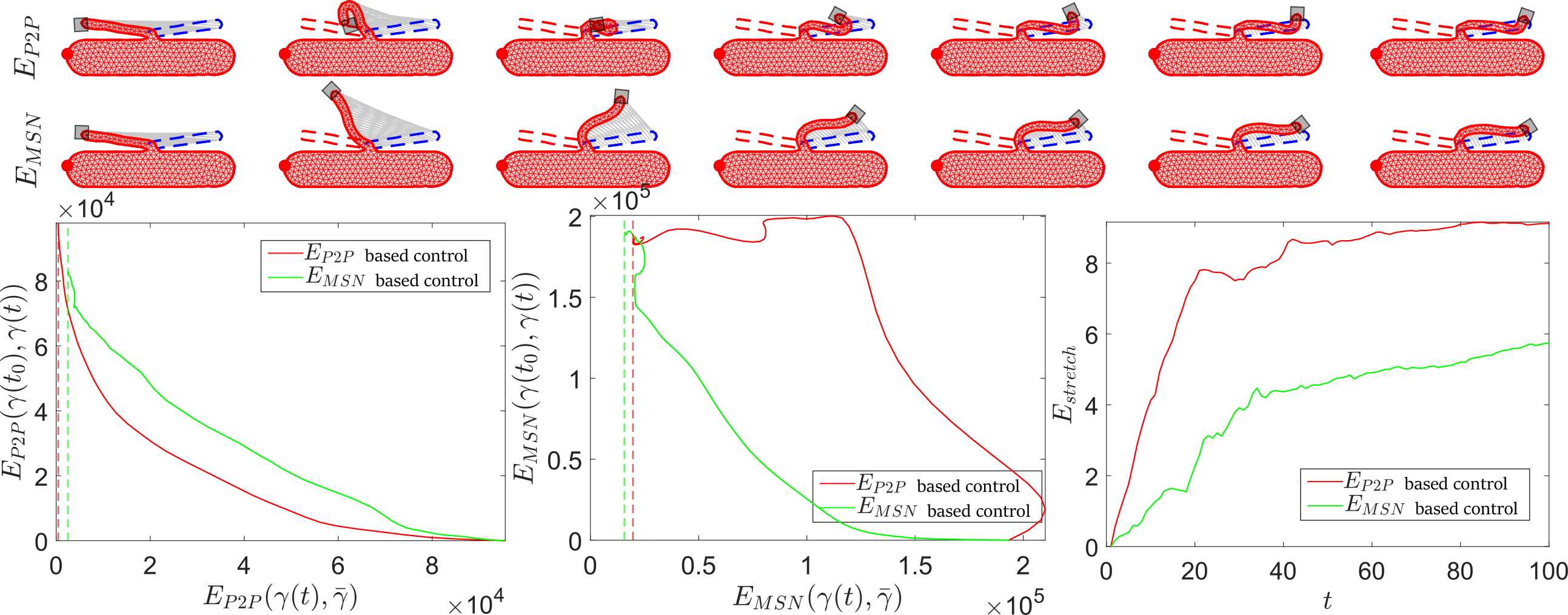
Given lemma ref, either \(E_{\mathrm{P2P}}\) in (5) or \(E_{\mathrm{FT}}\) in (6) serve to illustrate the importance of \(E_{\mathrm{MSN}}\) being an intrinsic and extrinsic metric for OCSC. In order to provide a better insight on the characteristics of \(E_{\mathrm{MSN}}\) as object-compliant shape metric, a comparison between two simulations is illustrated in Fig. 4. The first simulation seeks to reduce the extrinsic energy \(E_{\mathrm{P2P}}(\gamma(t),\bar{\gamma})\) whereas the second simulation reduces \(E_{\mathrm{MSN}}(\gamma(t),\bar{\gamma})\). The control strategy based on the reduction of \(E_{\mathrm{MSN}}\) leads to lower measured deformation as illustrated in the plots of Fig. 4. Moreover, the deformation cost expressed in terms of \(E_{\mathrm{MSN}}(\gamma(t_0),\gamma(t))\) is representative of the deformation values obtained from the simulation (unlike deformation cost expressed as \(E_{\mathrm{P2P}}(\gamma(t_0),\gamma(t))\)).
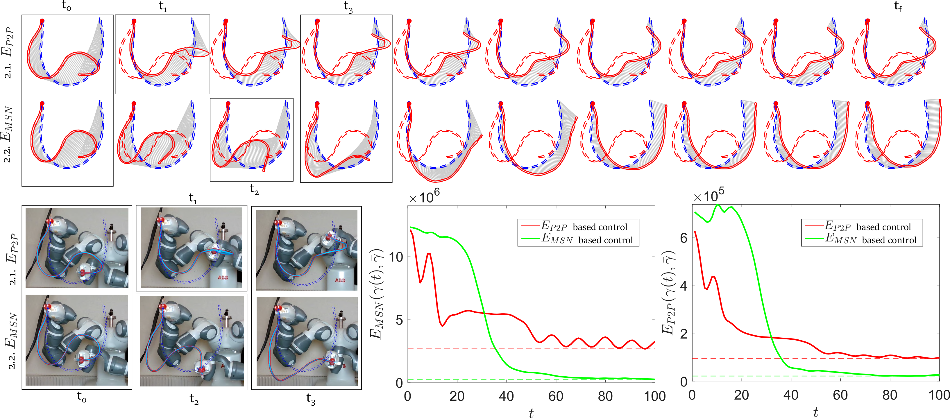
To further illustrate how our shape metric \(E_{\mathrm{MSN}}(\gamma(t),\bar{\gamma})\) inherently reduces not only the compression/extension strain but also the bending processes, in Fig. 5 we present Exp. 2.1 and Exp. 2.2. They involve the manipulation of an Ethernet cable that cannot be stretched or compressed (pure isometric deformations). Strategies based on the reduction of \(E_{\mathrm{P2P}}(\gamma(t),\bar{\gamma})\) and \(E_{\mathrm{MSN}}(\gamma(t),\bar{\gamma})\) are compared again in Exp. 2.1 and Exp. 2.2 respectively. This particular shape control problem constitutes a clear example of how seeking a local minimum in extrinsic energies such as \(E_{\mathrm{P2P}}(\gamma(t),\bar{\gamma})\) can lead to very large deformation processes that may even result in object self-intersections. See the high deformation and self-intersection of the cable in Exp. 2.1. On the other hand, the joint nature of \(E_{\mathrm{MSN}}(\gamma(t),\bar{\gamma})\) allows to untangle the cable and achieve a proper solution in Exp. 2.2. In Exp. 2.2 the intrinsic nature of the \(E_{\mathrm{MSN}}\) (SE(2) invariant) seeks to match the target contour's curvature regardless of its rigid configuration (position and orientation). That is, the strategy in Exp. 2.2 seeks object shape control rather than object position control, as Exp. 2.1 does.