Multi-scale Procrustes-based 3D shape control

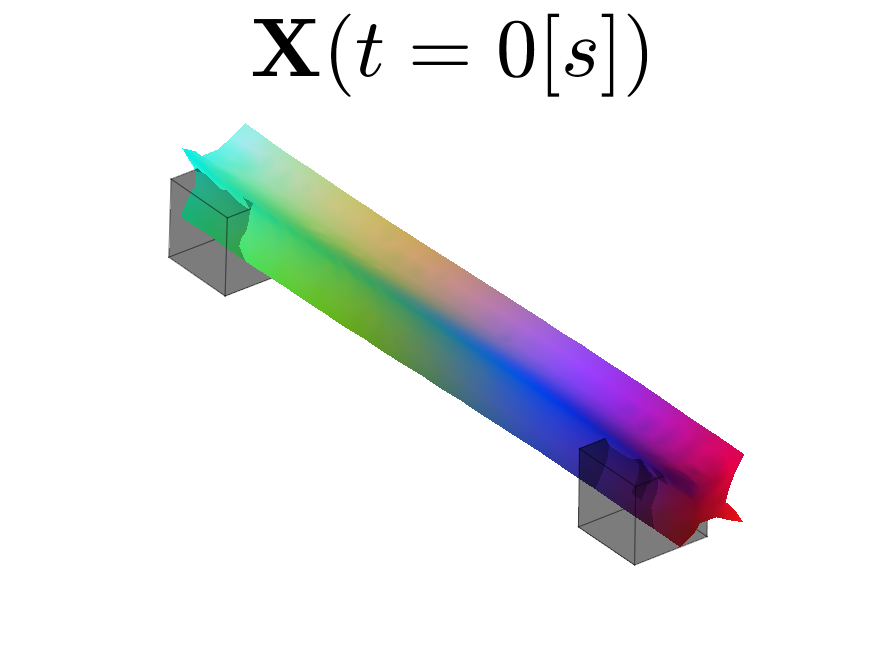
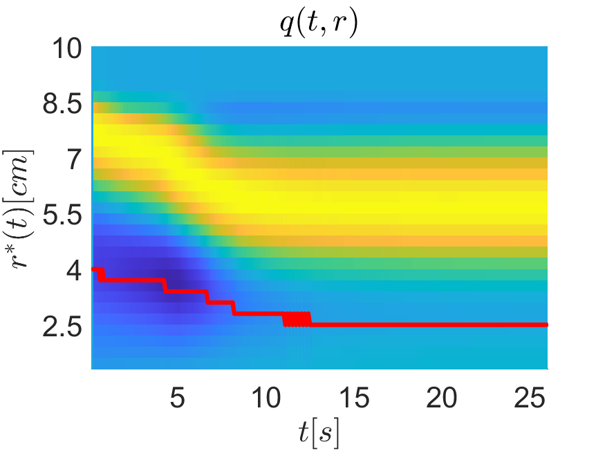
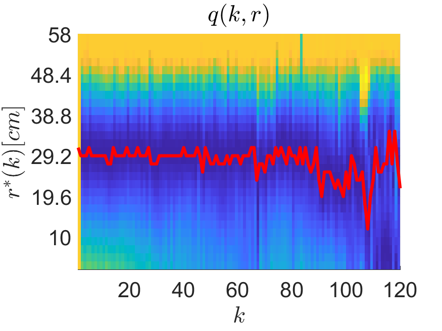
We performed several simulations using the ARAP (Sorkine and Alexa, 2007) deformation model. The simulation results are presented in Fig. 2. Within this figure, each column presents the results of a simulation. We normalised the colour map depicting values of \(q(t,r)\) so that negative values are blue, positive values are yellow and zero (or close to zero) values are green. One intuition for interpreting surface \(q(t,r)\) is to think of each scale \(r\in [ r_0 ,R(t)]\) (at a given instant \(t\)) as an available choice of an action to be performed under the relaxed LRB assumption. The value of \(q(t,r)\) (10) constitutes the error derivative estimation that each action will cause. Our method seeks large error reduction by choosing actions \(r^*(t)\) (11) that present large negative values of \(q(t,r^*(t))\).

The first simulation in Fig. 2 constitutes a challenging case given its anti-symmetry. This is specially noticeable in the last plot where surface \(q(t,r)\) presents estimations of positive error derivatives at large scales right at the initial configuration (\(t=0\), yellow tones around \(r=7\) [cm]). In other simulations, positive derivative estimations begin to appear later during the control process. Nonetheless, our initial choice of \(r^*(t_0)\) ensures \(q(t,r^*)<0\) and the control task is performed properly.

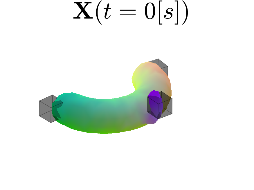
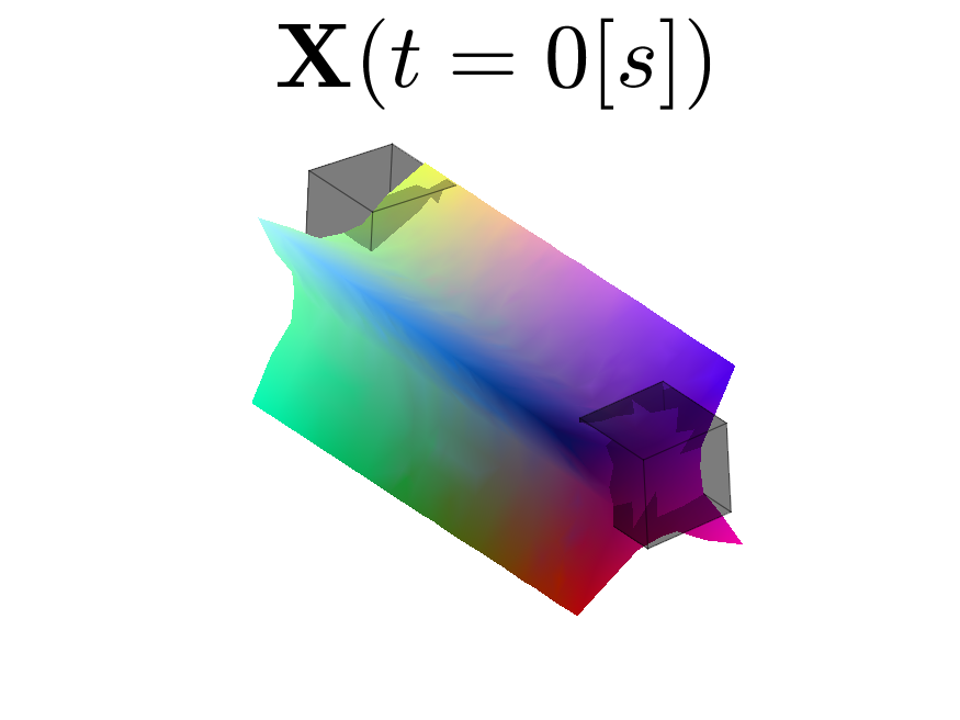
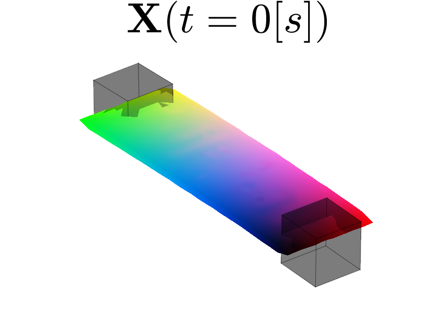
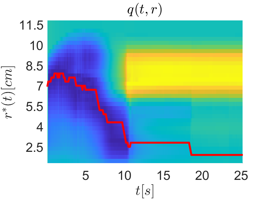
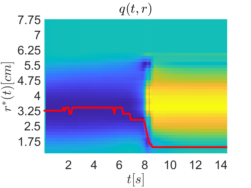
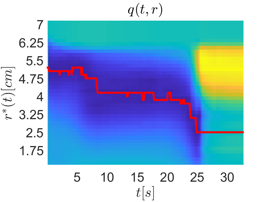
The simulation in the second column in Fig. 2 constitutes a paradigmatic example of how our multi-scale analysis works. Note how our strategy is able to prioritise larger elements of the object (i.e., larger \(r^*(t)\) values) when their contribution to the error term is large. The gripper positioned at the small appendix will collaborate in reducing the main beam error. Whenever the main beam error is reduced, the focus shall return to the reduction of the appendix' error (note the scale transition of \(r^*(t)\) between \(t=5\) and \(t=10\)). The third column in Fig. 2 involves a pure-twist. This can be challenging given singularities of the opposed rotation actions. However, actions are defined symmetrically and the error is smoothly reduced. Fourth column in Fig. 2 constitutes an example of pure bending process. Additional simulations are shown in the attached video.

We present several experiments (Fig. 3) with deformation cases analogous to those shown in the simulations. Our setup consists of two ABB IRB120 industrial robots (equipped with pneumatic grippers) and an Intel Realsense D415 RGB-D camera that provides the depth information we use for the 3D analysis. The objects to be handled are single-coloured foam cut-outs that favour colour-based segmentation. Recall that our method is designed for relatively rigid objects that align with our local-rigidity behaviour assumption. Therefore, we cannot guarantee its proper performance with softer objects, such as clothes. The analysis is carried out in Matlab and the communication with the robots is via TCP/IP. To avoid dropping below the process frequency of 5 Hz with the previously mentioned set-up, we propose discretising \(r\) to a set of around 20 scale values. Note that, given the analysis in Appendix A, \(q(r,t)\) in (11) is continuous differentiable. Therefore, using discrete points to approximate partial derivatives of \(q(r,t)\) by means of classic methods (e.g., polynomial regression) holds mathematical significance. Regarding the code implementation, experiments were conducted on an Intel(R) Core(TM) i7-8565U CPU with 1.99 GHz and 16 GB of RAM ^[1].

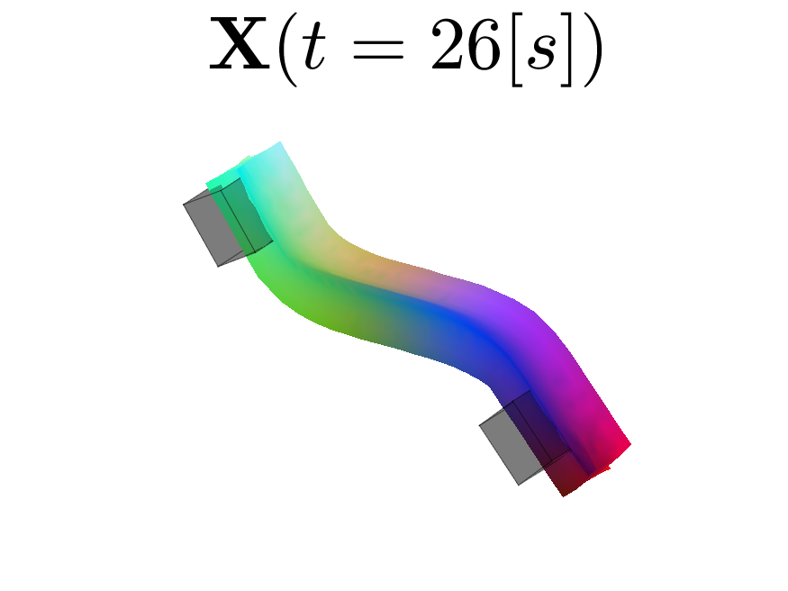
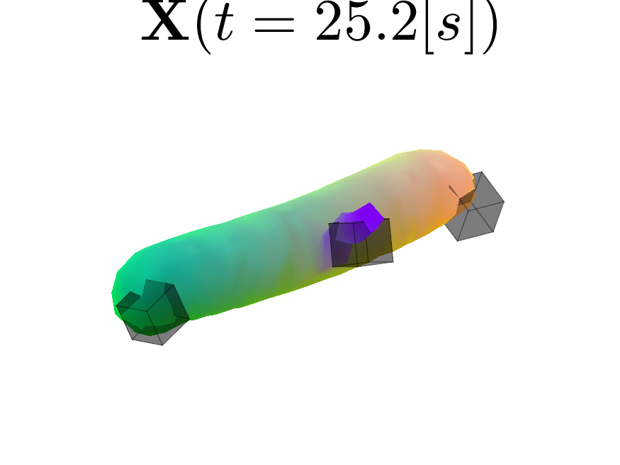
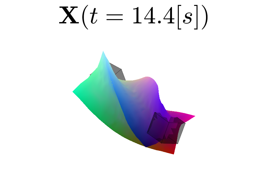
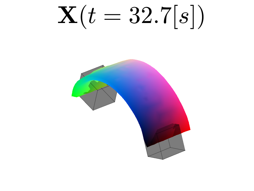
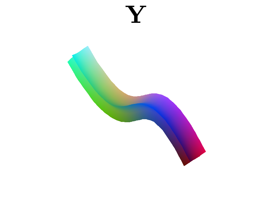
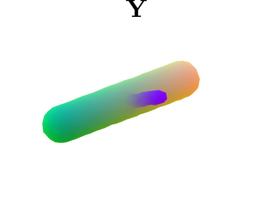
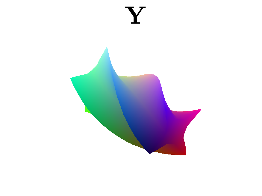
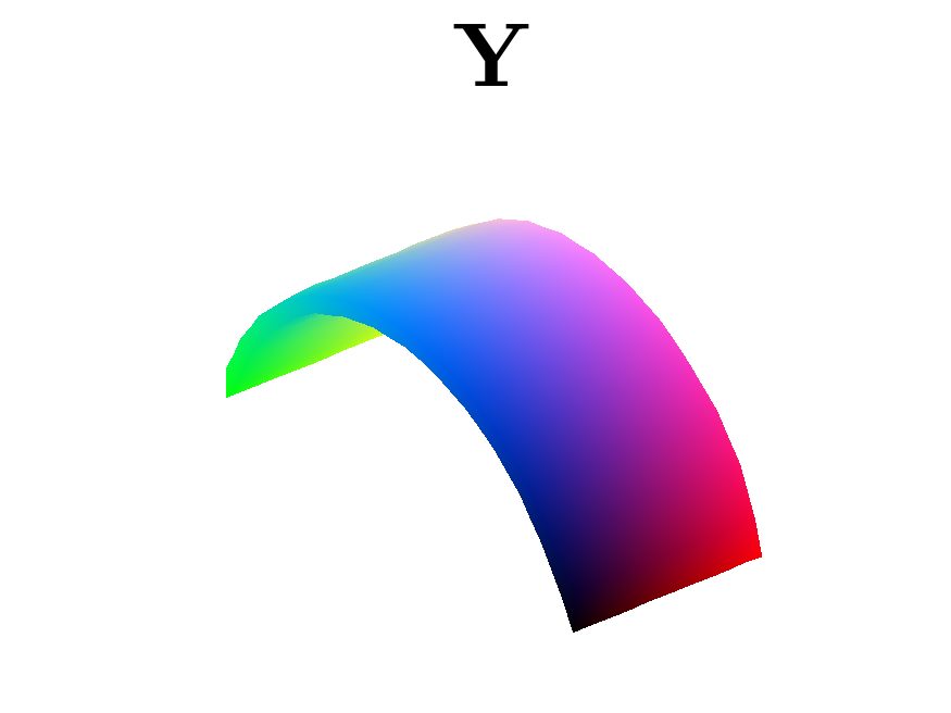
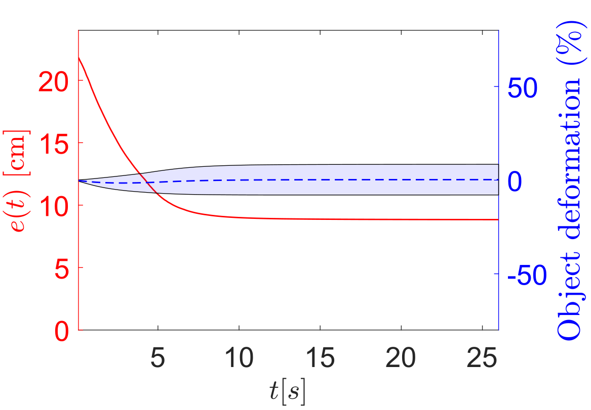
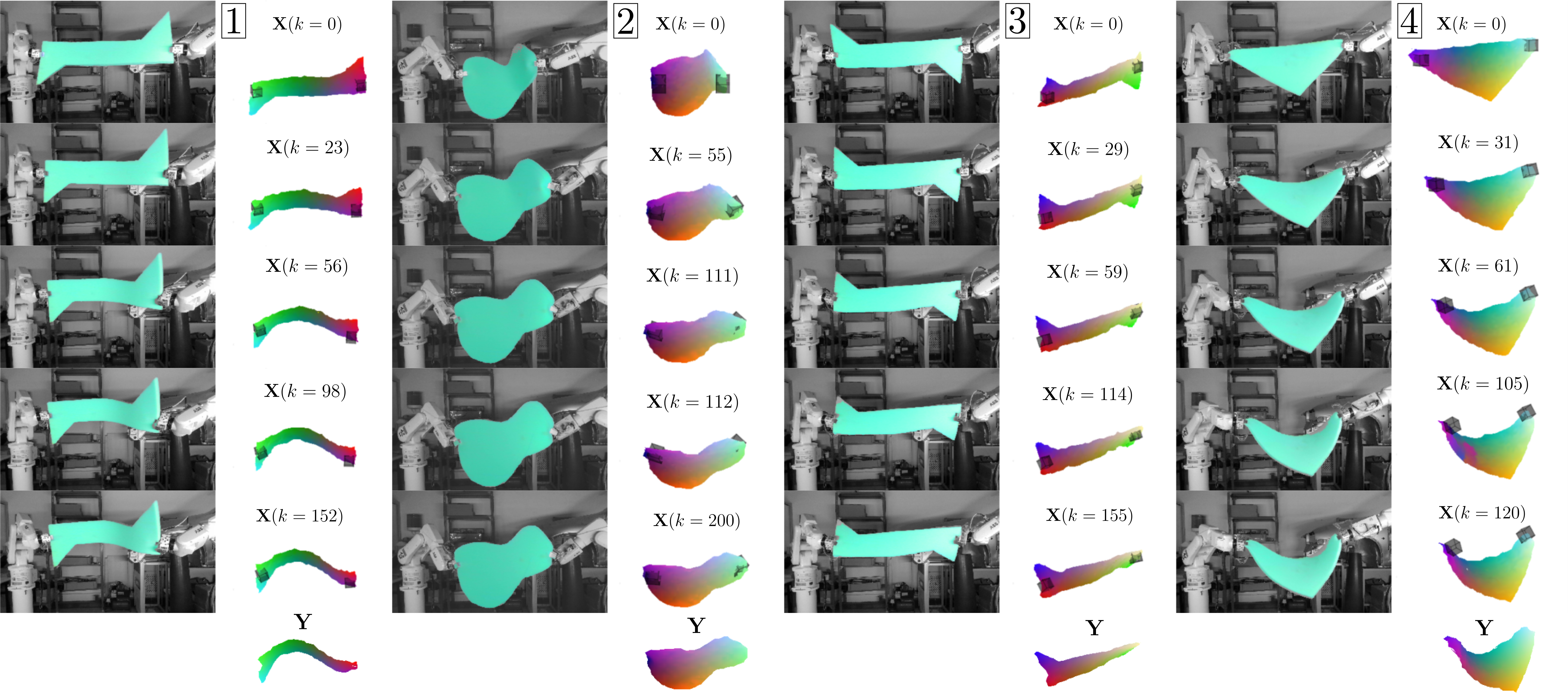
All shape control problems tackled in the experiments involve 3D surfaces. Target shapes have been pre-defined with robot configurations that ensure that the shape is achievable; this ensures, for example, that the robot is not required to leave its workspace. The setup, the object-segmentation and several relevant time instants are shown in Fig. 3. For each of the four experiments several acquired RGB images are shown grayscale along with the object segmentation highlighted in blue. The object's 3D points (corresponding to each time instant) are shown from a slightly elevated viewpoint that provides a better understanding of the 3D configuration of the object. The grippers are represented with gray cubes, and the target shape \(\mathbf{Y}\) with the surface mapping (colour map on the object) is shown at the bottom of the sequence. The attached video presents several additional perspectives that provide a better insight of the 3D configurations of the objects.

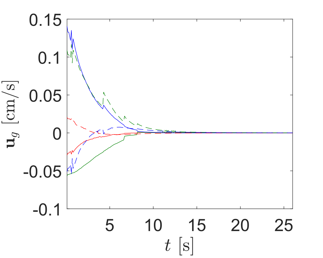
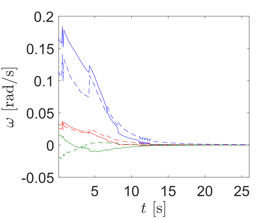
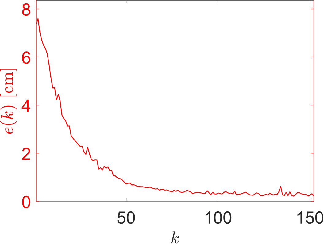
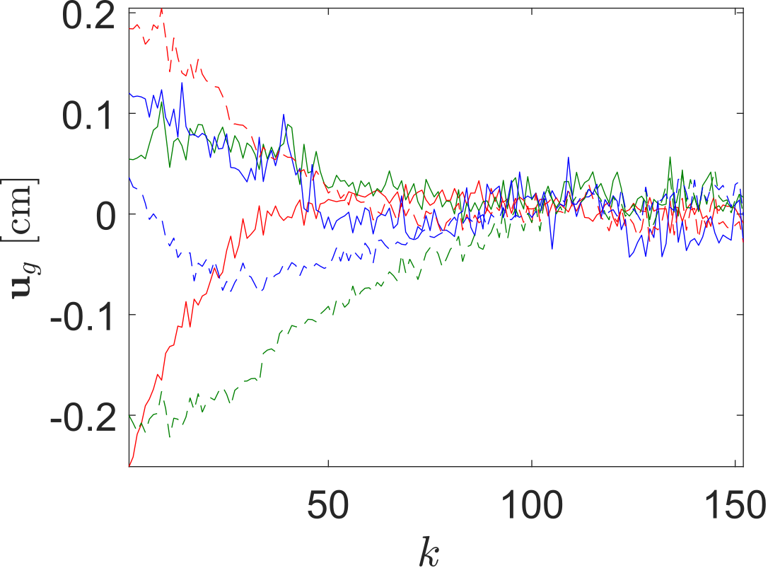
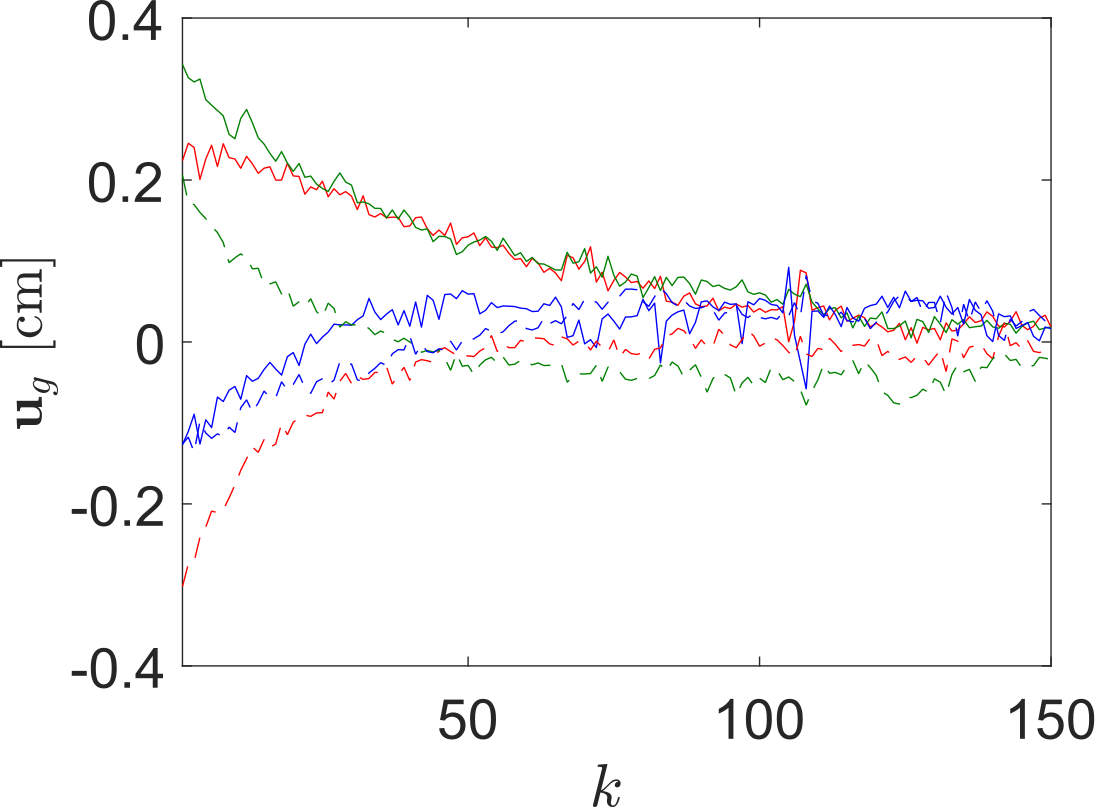
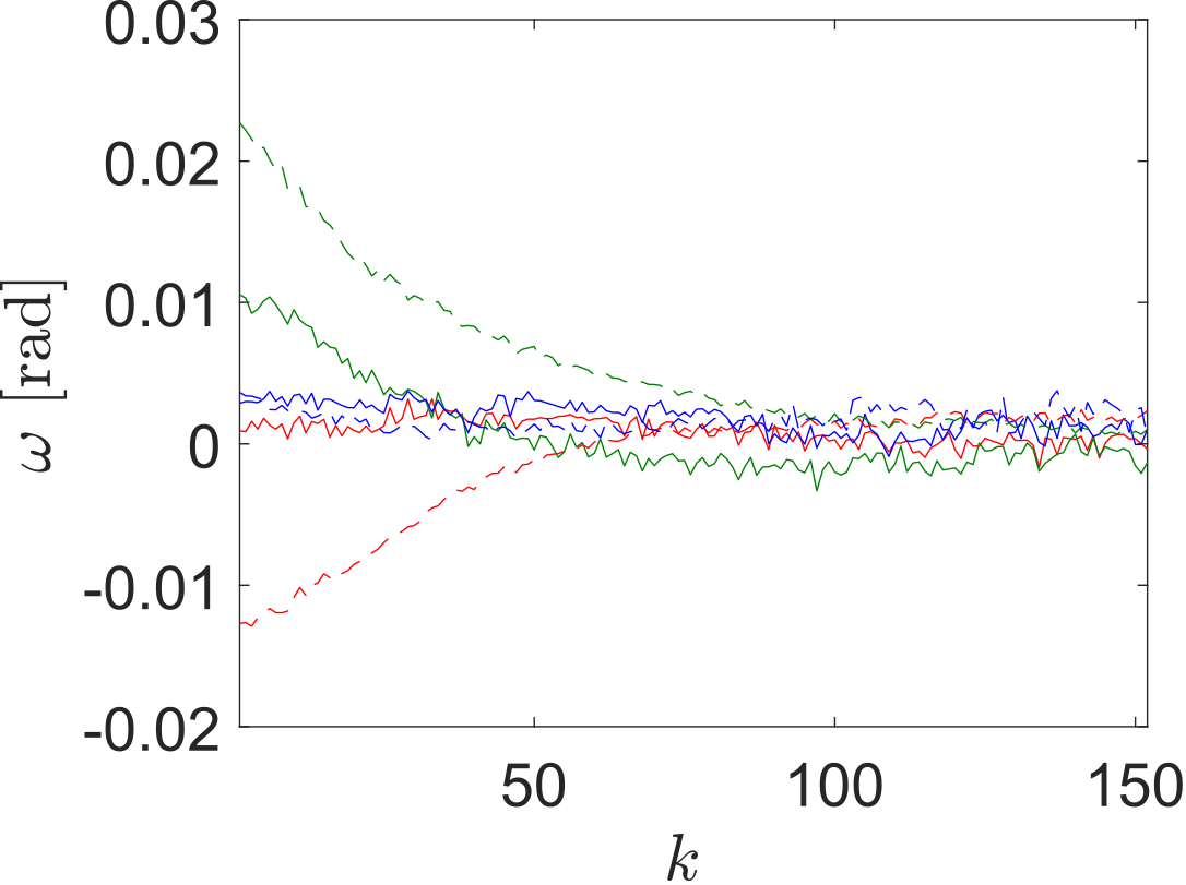
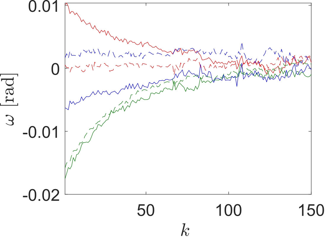
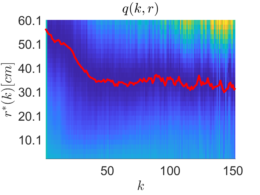
The first experiment in Fig. 3 involves an anti-symmetric bending process along with a light twist. A trend-change can be observed on the actions after \(k=20\), specially on the \(y\) and \(z\) components of \(\mathbf{u}_g\) (green and blue) and the \(y\) components of \(\mathbf{\omega}\) (green). This is a consequence of the evolution of \(r^*(k)\) during the first \(50\) iterations: our system focuses first on the bending process as it is responsible for larger error reduction and then tackles the twisting process.

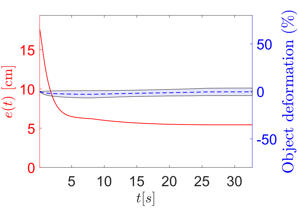
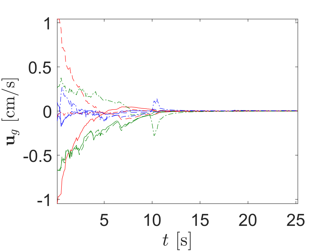
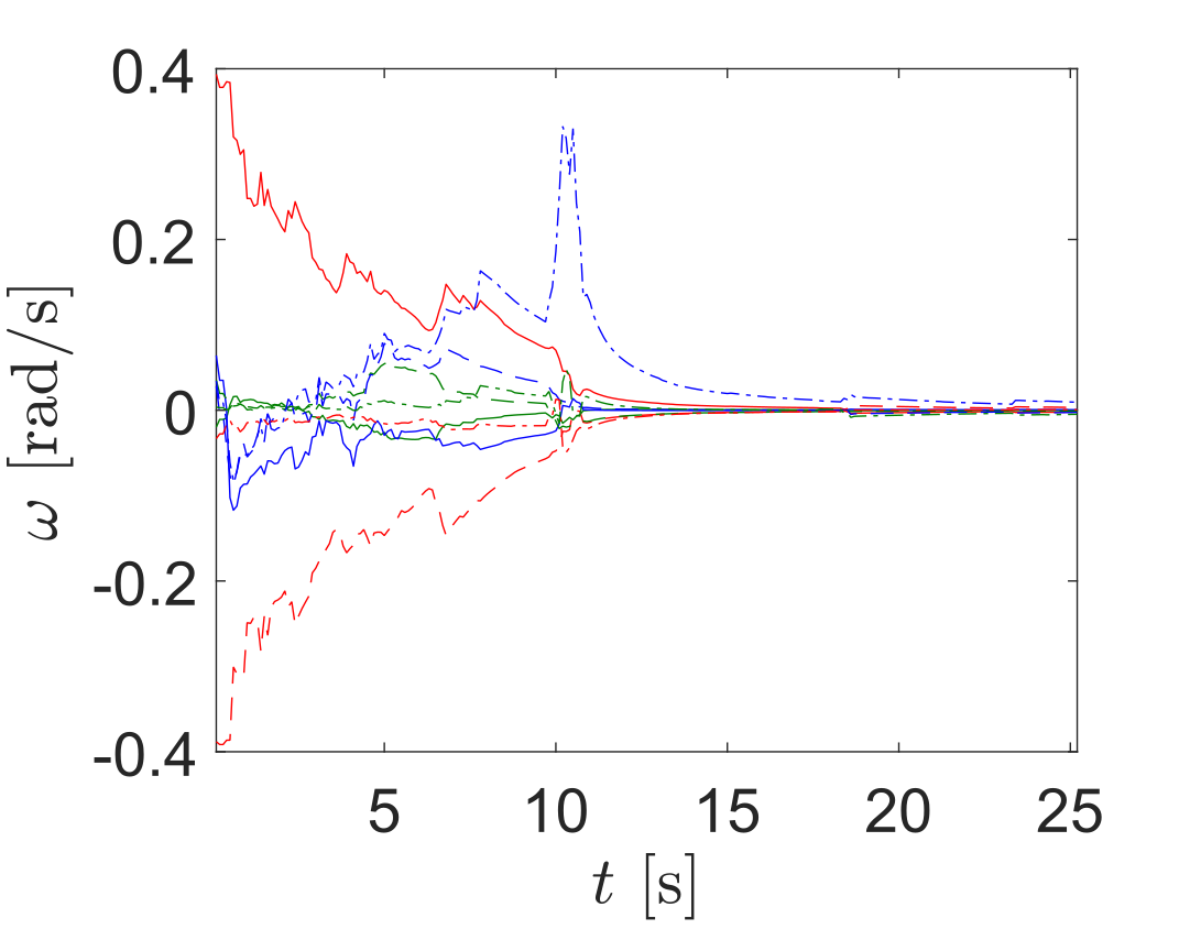
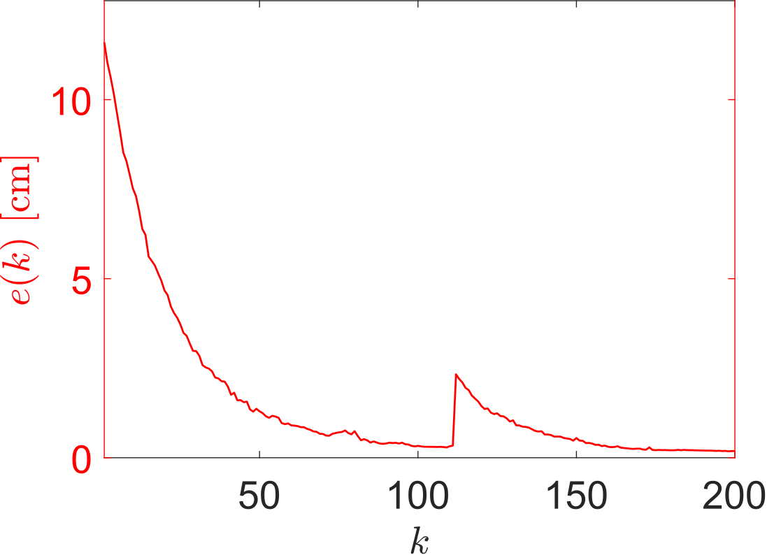
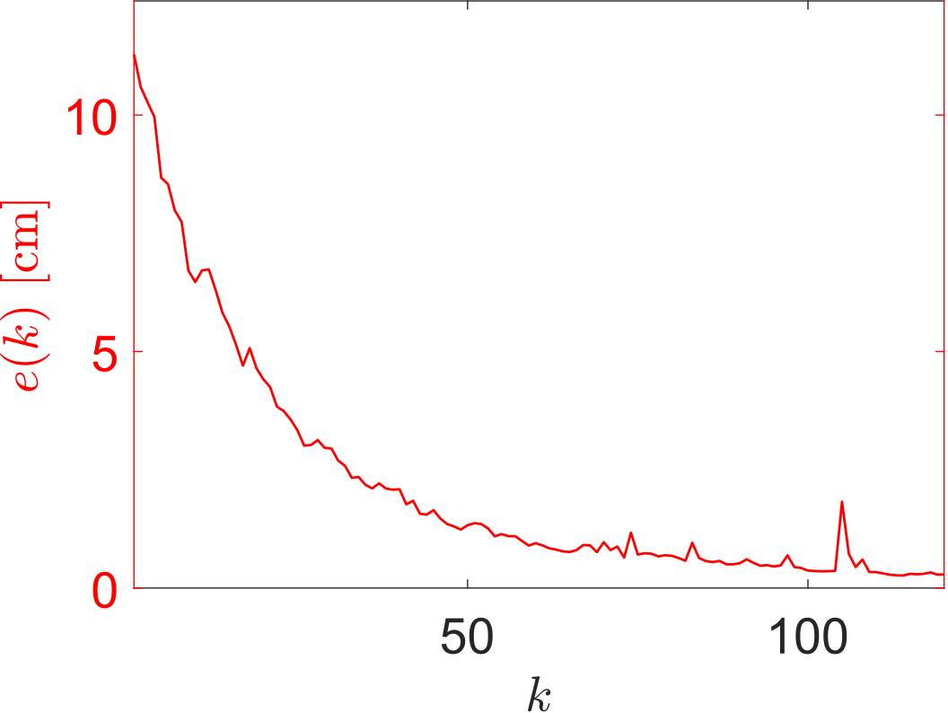
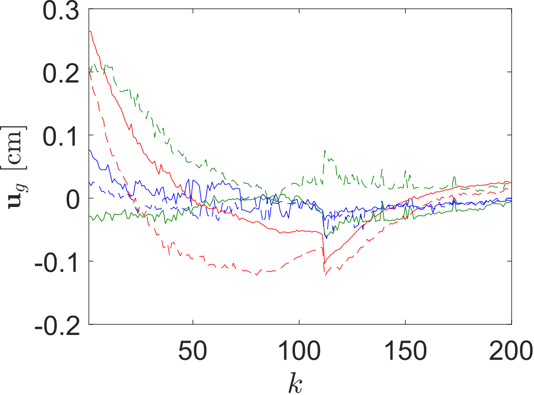
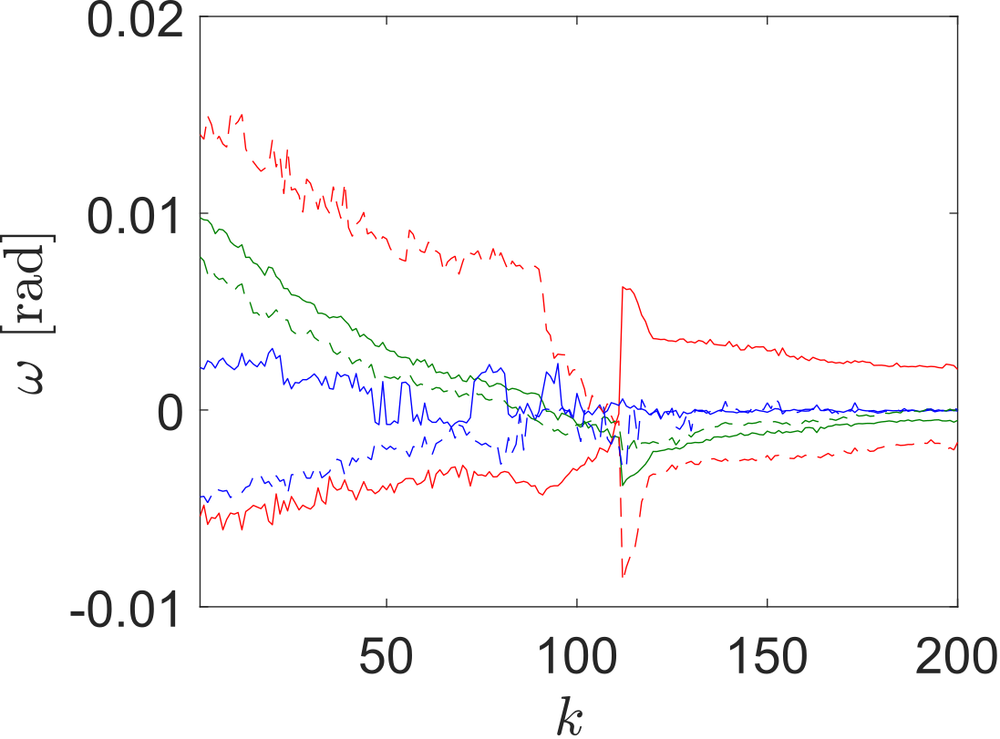
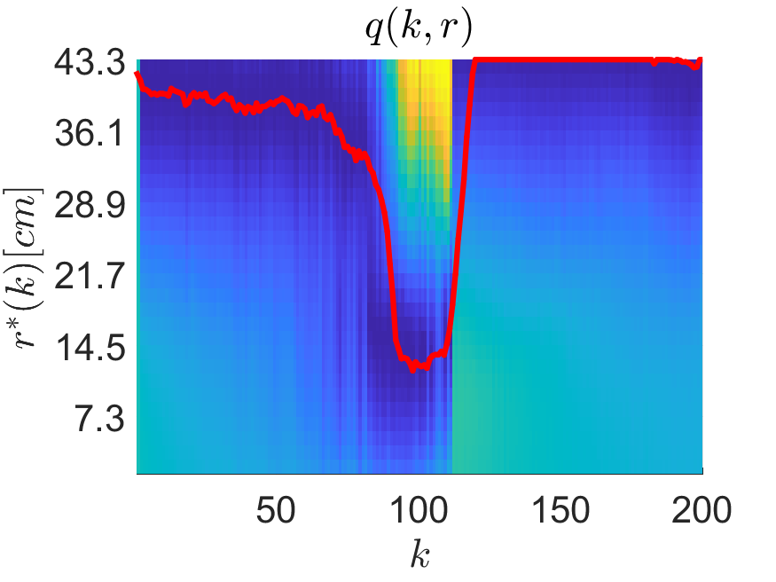
The second experiment consists of unfolding an object from a bent to a straightened configuration. This shape control problem is particularly challenging as, when approaching the target shape (around \(k=110\)) the object buckles thus breaking the assumption of small deformations between iterations and generating unreliable estimations of \(q(k,r)\). The buckling produces a global shape change on the object and thus \(r^*(k)\) undergoes an abrupt change towards global scale values (i.e., \(r^*(t)=R(t)\)). Even so, the system shows robustness and manages to continue converging. The buckling process can be better perceived in Fig. 3 and in the top view of the experiments video: between \(k=111\) and \(k=112\) the object suddenly changes its curvature with respect to the camera's front view.

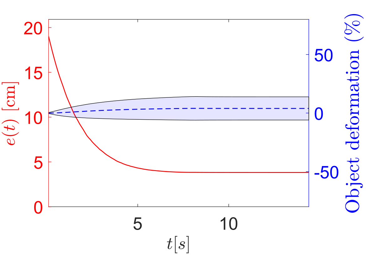
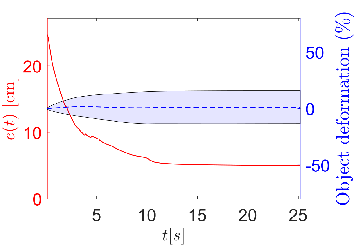
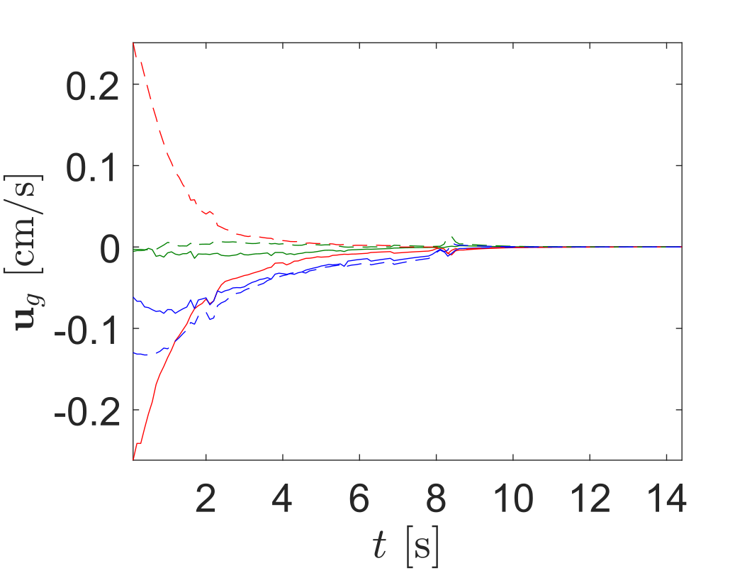
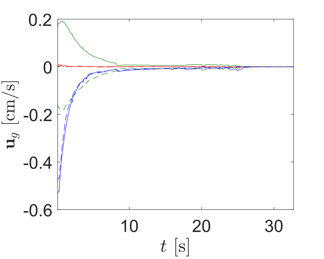
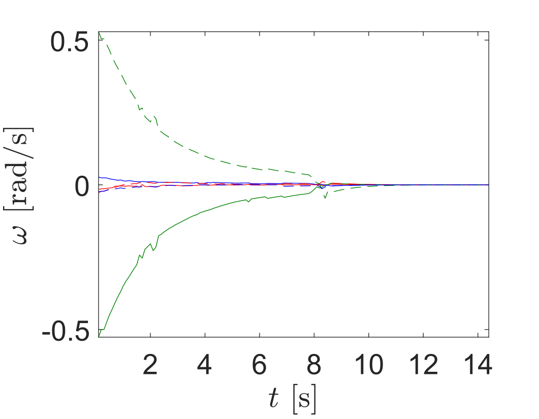
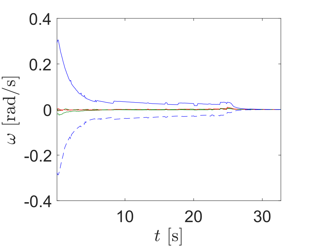
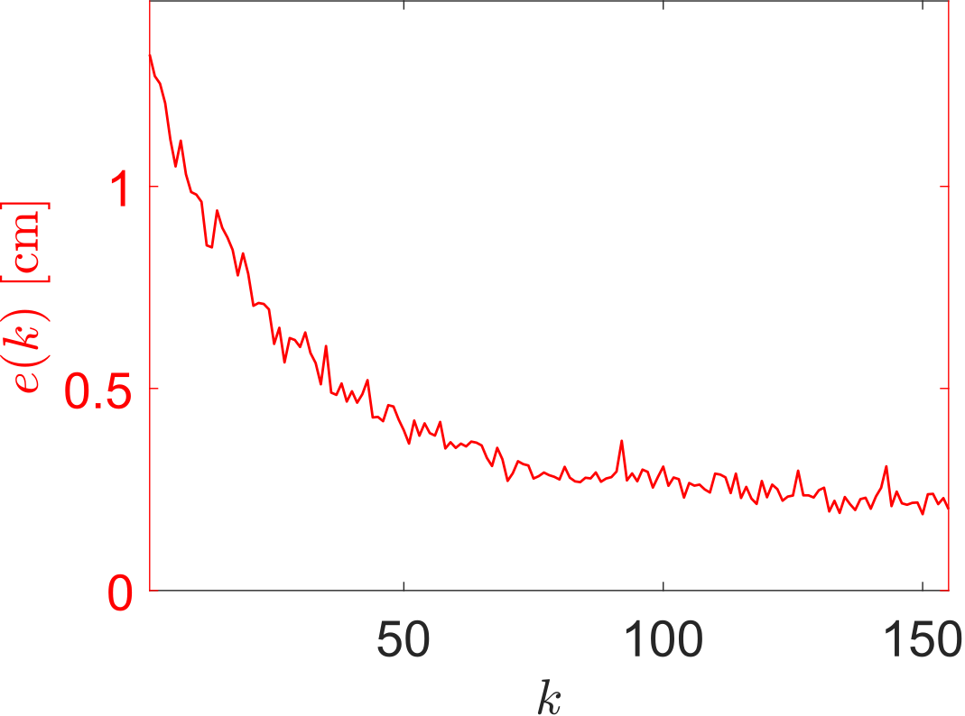
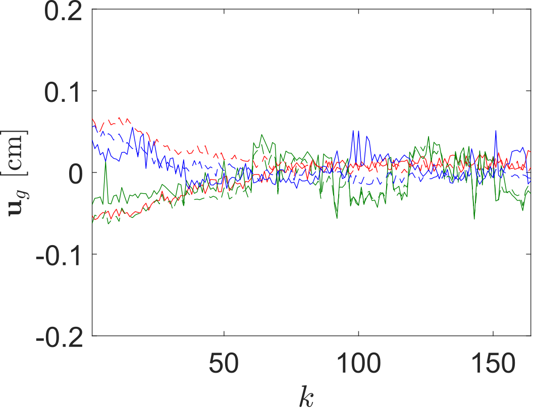
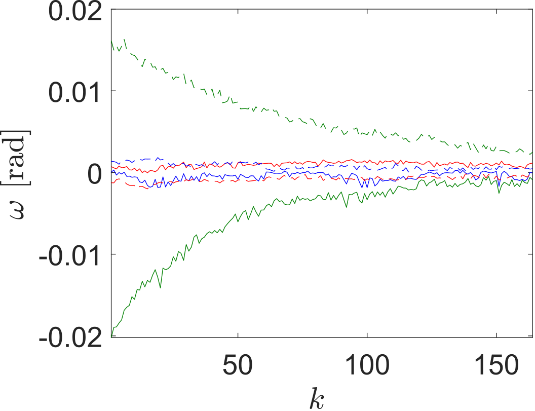
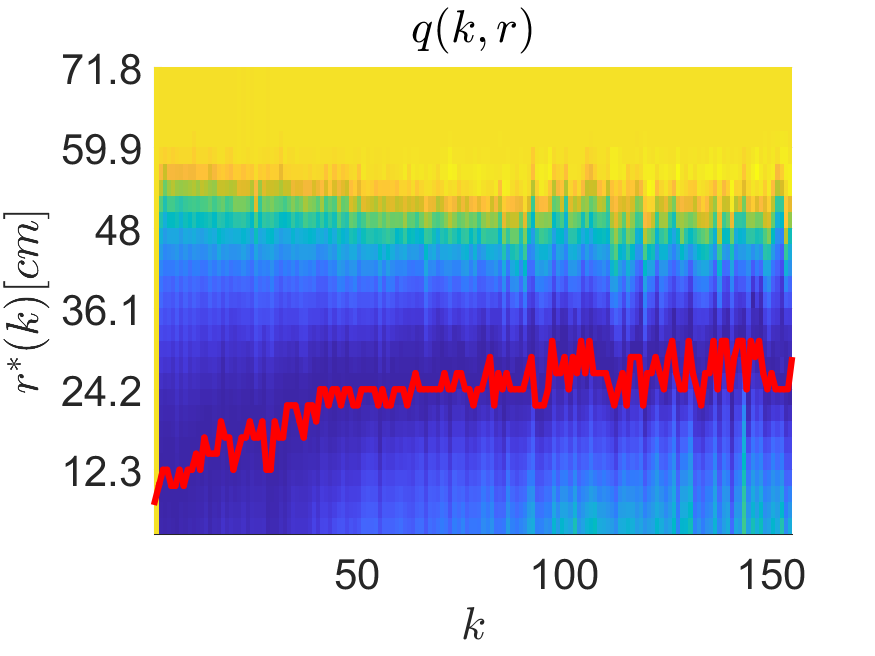
The third experiment in Fig. 3 involves a pure-twisting process. As in the analogue simulation, the alignment of the rotation axes can be problematic, as opposite rotation actions are coupled. Our control system generates symmetric rotation actions that evenly deform both sides of the object. Optimal scale \(r^*(t)\) increases as the object increases its rigidity due to the accumulated torsion: the object's response to pure rotation at larger scales takes some iterations. This is not the case in the analogous simulation, as the ARAP deformation model prioritises homogeneous deformation along the whole object from the initial time instant. The fourth experiment involves the 3D bending of a triangle shape. The shape control task is properly managed. However, it is worth mentioning a small error increase at \(k=105\). This is due to a discontinuity in the surface mapping that infringes the assumption of surface continuity. This lack of map-continuity can be appreciated in the last column of Fig. 3, where a colour map discontinuity can be observed on the left side of the triangle (\(k=105\)). As a result, peaks (outliers) around \(k=105\) can be observed in all the plots of the fourth column in Fig. 3.

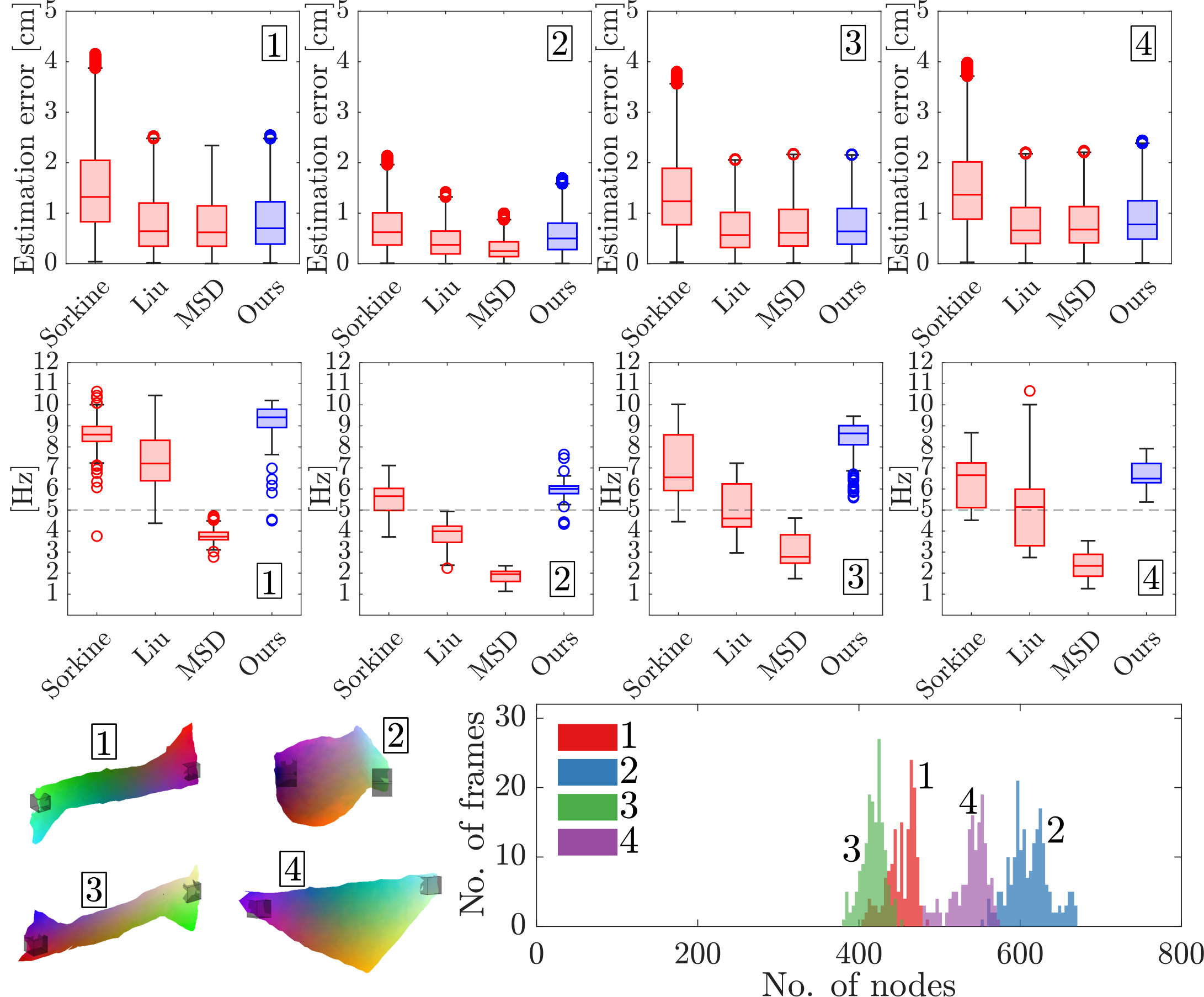
Fig. 4 shows the analysis of our proposed Procrustes-based deformation model regarding estimation error, computation frequency, and volume of analysed data. The estimation error is defined by comparing predicted and measured node positions during iterations. We compared our model against geometry-based deformation models from (Sorkine and Alexa, 2007) (used in (Shetab-Bushehri et al., 2022)(Shetab-Bushehri et al., 2022)) and (Liu et al., 2008), as well as a mass-spring-damper (MSD) physical-based model. Our model competes well with these three models, achieving a desirable balance between accuracy and computation time-cost. In addition, unlike the time cost of the other three models, our process' time cost also encompasses the cost of computing the control actions. The favourable balance between model accuracy and low computation time cost makes our model an attractive choice for shape control. Note that these comparisons do not aim to constitute conventional bench-marking: some aspects, such as the type of mesh or the set maximum number of optimisation iterations, may affect the performance of different deformation models in distinct manners. This makes it difficult to make fair comparisons. However, seeking fairness in the comparisons, we imposed a maximum limit of 20 iterations on the optimisation process for all of the compared models. This approach allows for a reasonable evaluation of model performance in shape control, despite the inherent complexities involved in comparing diverse methods.